Photon Research

Are we, as long-term investors, contributing to market predictability?

If you’ve ever experienced the Chinese college entrance exam – Gaokao, and attended a boarding school, you’ll know how important a predictable schedule can be.

Every day at 7 am, cheerful music plays through every dormitory, echoing down the halls and nudging everyone to wake up. At 11 pm sharp, the electricity cuts off. No lights, no devices, no distractions. Dorm guards stroll through the hallways for about 20 minutes, checking for any sneaky light or noise coming from rooms. It’s a strict routine designed to keep students focused, all for the students’ own good.

It is a form of behavioural discipline. If you can’t get out of the system, win within system.

After a while, students developed counterstrategies. Every day we get back to the dorm around 10 pm from our evening study, which gives us a perfect hour to prepare for the blackout.

Rechargeable lamps, little tents or curtains around our desks, and absolute silence during those first 20 minutes after the dark.

We managed to find a way to stay up late, because the rules were static and predictable.

Of course, today’s topic is not about sneaking past dorm rules. Today, I want to talk about an investment discipline – rebalancing of the portfolio, and the pattern of institutional funds carrying out such activity.

More specifically, can others anticipate and trade ahead of large, predictable flows, such as rebalancing by institutional investors like pension funds, particularly around month-end or quarter-end periods?

The intuition is straightforward: large institutions often follow mechanical rebalancing rules (monthly or quarterly), if enough market participants follow similar schedules and thresholds, their collective trading behaviour could become predictable. This, in turn, might create short-term price distortions around these times, especially at the end of the month or quarter.

If so, this raises a further question: should we alter our investment behaviour to avoid being front run? Should we create a certain level of uncertainty around our rebalancing behaviour?

Adjustable Assumptions

Before we start, it might be useful to look at a list of adjustable assumptions/inputs, which we can tune or iterate over to observe how sensitive the results are under different conditions:

• Rebalancing Frequency
  • Monthly or quarterly. Different investors may operate on different cycles
• Trading Windows
  • Define windows around the end and beginning of each month. We will refer to this as the “End of Month” (EOM) period, which could span 1 to 5 trading days on either side of the month boundary. All other days will be referred to as the “Rest of the Month” (ROM).
  • Unless otherwise specified, the default EOM window used in this analysis refers to the last trading day of each month.
• Rebalancing Thresholds
  • Institutional investors can tolerate some degree of drift to avoid excessive trading costs.
  • A drift threshold (e.g., 0% to 5%) can help model when a rebalance is likely to be triggered. For example, if the portfolio’s asset drifts by less than 5%, rebalancing may be skipped.
• Portfolio Composition
  • While a 60/40 (equity/bond) portfolio is commonly cited, this article uses a proxy based on market capitalization of major benchmarks. By using the MSCI USA Index and the Bloomberg US Aggregate Bond Index as proxies, we obtain a split closer to 65/35.
  • Admittedly this approach can be equally naïve

If a consistent EOM effect exists, it could suggest that institutional rebalancing creates small but repeatable market inefficiencies. In theory, active traders could exploit these flows by anticipating buying or selling pressure in certain asset classes.

Our Hypothesis

Trading volume and returns on the last trading day of each month are systematically different (higher volume, higher/lower returns) than other trading days, possibly due to fund rebalancing activities.

Boxplot

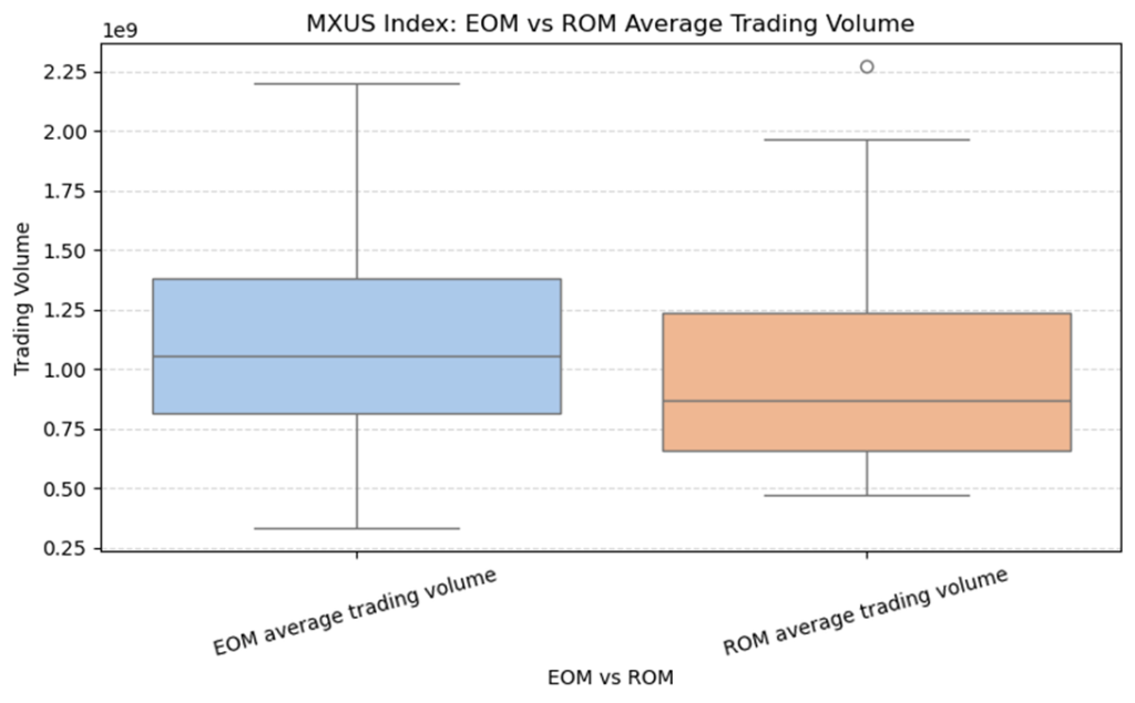
To start with, we generate a boxplot comparing trading volumes on:

• The trading days around the end of each month
• The average daily volume during the rest of the month

As shown in Exhibit 1, the boxplot visually confirms that average trading volume on EOM days is noticeably higher than the average volume during ROM days.

Statistical Test: T-Test

To verify whether these differences are statistically significant, we perform T-Tests comparing returns and trading volumes between EOM and ROM days.

• Absolute equity return comparison:
  • T-statistic: -2.566
  • P-value: 0.0107
• Trading volume comparison:
  • T-statistic: 4.950
  • P-value: 0.0000
• Excess return of equities over bonds within the portfolio:
  • T-statistic: -2.014
  • P-value: 0.0448

Excess return of equities over bonds within the portfolio measures the relative performance of equities compared to fixed income, based on a weighted portfolio (e.g., 65/35 equity/bond), i.e. equity drift.

The results show a statistically significant difference in average returns and average excess returns between EOM and ROM days and confirms that trading volumes on EOM days are consistently and significantly higher than during the rest of the month.

Rolling correlation

We compute a 21-trading-day (approximately one month) rolling correlation between log trading volume and excess return. To highlight potential patterns around rebalancing activity, we flag the last two and first two trading days of each month as the EOM trading window, creating a 4-day span surrounding the month-end boundary.

While the analysis can extend further back, we focus on a recent sample period for better visual clarity. In the chart below, red dots represent EOM trading windows. Notably, these markers often appear near the peaks or troughs of the rolling correlation line. This suggests that the correlation between volume and excess return tends to spike, either positively or negatively, around EOM periods. In other words, return is more sensitive to volume swings during these windows, consistent with rebalancing-related activity. Since excess return can be both positive and negative, this heightened correlation (in absolute terms) aligns with the idea of increased trading pressure during rebalancing.

Regression analysis 1

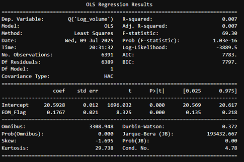
We introduced a binary indicator variable—set to 1 if the data point corresponds to an EOM day, and 0 otherwise. We then ran a simple regression model:

Volume = β₀ + β₁ × EoM Flag + ε

Result suggests thaton average, log volume is statistically significant higher by 0.1767 on EOM days.

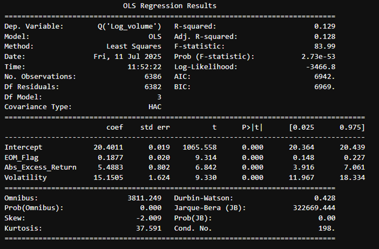
Next, we introduce control variables into the regression: the excess return of equities over bonds and the 5-day (one-week) volatility:

Volume ~ EOM Flag + Excess Return + Volatility

The results provide strong statistical evidence that EOM volume remains about 20% higher even after controlling for these factors (exp(0.1815) ≈ 1.20,  ~20% higher).

Interestingly, excess return and volume are inversely related, while absolute excess return shows a positive correlation with volume, suggesting that large relative moves, regardless of direction, increase trading activity.

As expected, volatility is a major driver of volume, with a strong and statistically significant positive effect: higher volatility (e.g., fear or uncertainty) increases trading activity.

Regression analysis 2

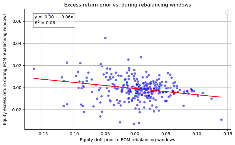
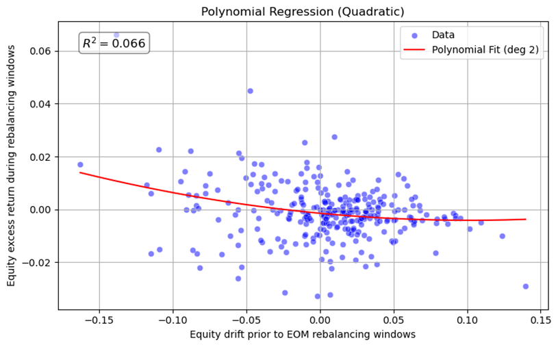
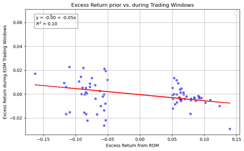
We then run a regression using equity drift prior to the EOM rebalancing window as the independent variable, and the excess return of equities during or immediately after the rebalancing window as the dependent variable.

Excess Return (EOM) = β₀ + β₁ × Equity Drift (ROM) + ε

The results, shown in the chart below, suggest a statistically significant inverse relationship: when equities outperform fixed income earlier in the month, creating upward drift, returns during the rebalancing window tend to be lower, and vice versa. This inverse relationship is statistically strong but explains only a modest portion of the variance.

To account for potential non-linearity, we also perform a quadratic polynomial regression.

Regression analysis 3

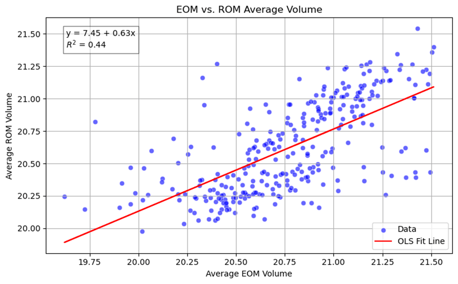
We then run a regression to observe trading volume.

Trading Volume (EOM) = β₀ + β₁ × Trading Volume (ROM) + ε

ROM trading volume appears to drive EOM trading volume, which is intuitive – higher trading activity throughout the month tends to be associated with elevated trading volumes around month-end.

Regression analysis 4

Introducing a 5% tolerance threshold for rebalancing reduces the sample size, but the relationship remains broadly unchanged.

Final thoughts

Our findings suggest that there are observable differences in both returns and trading volume during end-of-month (EOM) rebalancing windows, supporting the view that long-term multi-asset investors may benefit from shifting their rebalancing schedules away from month-end to avoid potential crowding effects.

However, there is insufficient evidence to suggest that these flows can be reliably exploited for profit. To further develop robust signals and strategy, additional data, such as ETF flows, mutual fund flows, or other institutional activity reports from public research sources, would be necessary.

Disclaimer:
The views and opinions expressed in this blog are solely my own and do not represent the views of my employer or any affiliated organisation. The content is for informational and educational purposes only and is based on publicly available data.

This blog does not constitute financial advice, investment recommendations, or an offer or solicitation to buy or sell any financial instrument. No part of this content should be considered a financial promotion under the Financial Services and Markets Act 2000.

While care has been taken to ensure the accuracy of the information presented, I make no representations or warranties as to its completeness or accuracy and accept no liability for any errors or omissions. Please conduct your own research or consult a qualified professional before making any financial decisions.

Data Source: Bloomberg